45 how to put data labels in excel chart

How do you put values over a simple bar chart in Excel? Assuming you're using Excel 2007, data labels are added through the "Data Labels" selection. As shown below, cells A2:A5 contain the data Items. Cells B2:B5 contain the data Values. 1) Select cells A2:B5 . 2) Select "Insert" 3) Select the desired "Column" type graph. 4) Click on the graph to make sure it is selected, then select "Layout" Excel Charts: Creating Custom Data Labels - YouTube In this video I'll show you how to add data labels to a chart in Excel and then change the range that the data labels are linked to. This video covers both W...

Custom Chart Data Labels In Excel With Formulas - How To Excel At Excel Follow the steps below to create the custom data labels. Select the chart label you want to change. In the formula-bar hit = (equals), select the cell reference containing your chart label's data. In this case, the first label is in cell E2. Finally, repeat for all your chart laebls.

How to put data labels in excel chart

How can I hide 0% value in data labels in an Excel Bar Chart I would like to hide data labels on a chart that have 0% as a value. I can get it working when the value is a number and not a percentage. I could delete the 0% but the data is going to change on a daily basis. I am doing a if statement to calculate which column to put the data into.Data is shown below I have 2 bars one green and one red. Add or remove data labels in a chart - support.microsoft.com Click the data series or chart. To label one data point, after clicking the series, click that data point. In the upper right corner, next to the chart, click Add Chart Element > Data Labels. To change the location, click the arrow, and choose an option. If you want to show your data label inside a text bubble shape, click Data Callout. Edit titles or data labels in a chart - support.microsoft.com On a chart, click one time or two times on the data label that you want to link to a corresponding worksheet cell. The first click selects the data labels for the whole data series, and the second click selects the individual data label. Right-click the data label, and then click Format Data Label or Format Data Labels.

How to put data labels in excel chart. Prevent Overlapping Data Labels in Excel Charts - Peltier Tech May 24, 2021 · Overlapping Data Labels. Data labels are terribly tedious to apply to slope charts, since these labels have to be positioned to the left of the first point and to the right of the last point of each series. This means the labels have to be tediously selected one by one, even to apply “standard” alignments. How to add data labels from different column in an Excel chart? Right click the data series in the chart, and select Add Data Labels > Add Data Labels from the context menu to add data labels. 2. Click any data label to select all data labels, and then click the specified data label to select it only in the chart. 3. Change the format of data labels in a chart To get there, after adding your data labels, select the data label to format, and then click Chart Elements > Data Labels > More Options. To go to the appropriate area, click one of the four icons ( Fill & Line, Effects, Size & Properties ( Layout & Properties in Outlook or Word), or Label Options) shown here. How To Add Data Labels In Excel ~ Pvkngcchittoor Then, click the insert tab along the top ribbon and click the insert scatter (x,y) option in the charts group. Click on the arrow next to data labels to change the position of where the labels are in relation to the bar chart. To format data labels in excel, choose the set of data labels to format. Source:

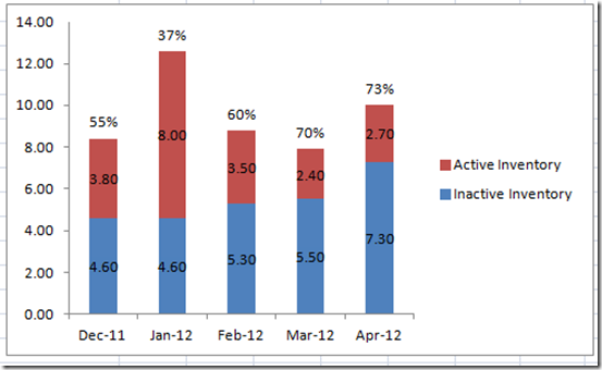
Excel charts: add title, customize chart axis, legend and ... Oct 29, 2015 · Click the Chart Elements button, and select the Data Labels option. For example, this is how we can add labels to one of the data series in our Excel chart: For specific chart types, such as pie chart, you can also choose the labels location. For this, click the arrow next to Data Labels, and choose the option you want. How to Add Total Data Labels to the Excel Stacked Bar Chart Step 4: Right click your new line chart and select "Add Data Labels" Step 5: Right click your new data labels and format them so that their label position is "Above"; also make the labels bold and increase the font size. Step 6: Right click the line, select "Format Data Series"; in the Line Color menu, select "No line" HOW TO CREATE A BAR CHART WITH LABELS ABOVE BAR IN EXCEL - simplexCT In the chart, right-click the Series "Dummy" Data Labels and then, on the short-cut menu, click Format Data Labels. 15. In the Format Data Labels pane, under Label Options selected, set the Label Position to Inside End. 16. Next, while the labels are still selected, click on Text Options, and then click on the Textbox icon. 17. How to Create Charts in Excel (In Easy Steps) - Excel Easy 1. Select the chart. 2. Click the + button on the right side of the chart, click the arrow next to Legend and click Right. Result: Data Labels. You can use data labels to focus your readers' attention on a single data series or data point. 1. Select the chart. 2. Click a green bar to select the Jun data series. 3.

How to add or move data labels in Excel chart? - ExtendOffice 1. Click the chart to show the Chart Elements button . 2. Then click the Chart Elements, and check Data Labels, then you can click the arrow to choose an option about the data labels in the sub menu. See screenshot: How to Add Two Data Labels in Excel Chart (with Easy Steps) Step 4: Format Data Labels to Show Two Data Labels. Here, I will discuss a remarkable feature of Excel charts. You can easily show two parameters in the data label. For instance, you can show the number of units as well as categories in the data label. To do so, Select the data labels. Then right-click your mouse to bring the menu. How to Change Excel Chart Data Labels to Custom Values? May 05, 2010 · Now, click on any data label. This will select “all” data labels. Now click once again. At this point excel will select only one data label. Go to Formula bar, press = and point to the cell where the data label for that chart data point is defined. Repeat the process for all other data labels, one after another. See the screencast. Excel: How to Create a Bubble Chart with Labels - Statology Step 3: Add Labels. To add labels to the bubble chart, click anywhere on the chart and then click the green plus "+" sign in the top right corner. Then click the arrow next to Data Labels and then click More Options in the dropdown menu: In the panel that appears on the right side of the screen, check the box next to Value From Cells within ...

| Pryor Learning Solutions

HOW TO CREATE A BAR CHART WITH LABELS INSIDE BARS IN EXCEL - simplexCT In the chart, right-click the Series "# Footballers" Data Labels and then, on the short-cut menu, click Format Data Labels. 8. In the Format Data Labels pane, under Label Options selected, set the Label Position to Inside End. 9. Next, in the chart, select the Series 2 Data Labels and then set the Label Position to Inside Base. 10.

Multiple bar charts on one axis in excel - Super User

I want to be able to hide the main data but have a separate tab where ... On the Optional features page, choose Next. At the top of the report from the drop-down menu, click on Excel to open the Excel report window. To create a new Excel workbook, click on the radio button beside "new Excel workbook". Otherwise, click on "existing excel workbook" to update an old one. If working on an already existing workbook, click ...

Improve your X Y Scatter Chart with custom data labels

How to create Custom Data Labels in Excel Charts - Efficiency 365 Create the chart as usual. Add default data labels. Click on each unwanted label (using slow double click) and delete it. Select each item where you want the custom label one at a time. Press F2 to move focus to the Formula editing box. Type the equal to sign. Now click on the cell which contains the appropriate label.

[5 Steps] How To Make Ranking Charts With Excel Pivot Tables - Moz

Create Dynamic Chart Data Labels with Slicers - Excel Campus Feb 10, 2016 · Typically a chart will display data labels based on the underlying source data for the chart. In Excel 2013 a new feature called “Value from Cells” was introduced. This feature allows us to specify the a range that we want to use for the labels. Since our data labels will change between a currency ($) and percentage (%) formats, we need a ...

How to Change Excel Chart Data Labels to Custom Values? | Chandoo.org - Learn Microsoft Excel Online

How to Add Data Labels to your Excel Chart in Excel 2013 Watch this video to learn how to add data labels to your Excel 2013 chart. Data labels show the values next to the corresponding ch...

How To Add A Title To A Table In Excel | Decoration Drawing

How To Create Labels In Excel - pelautindonesia.info Make Row Labels In Excel 2007 Freeze For Easier Reading from . Starting document near the bottom. Click a data label one time to select all data labels in a data series or two times to select just one data label that you want to delete, and then press delete. Click finish & merge in the finish group on the mailings tab.

Excel Chart Not Showing All Data Labels - Chart Walls

Add a DATA LABEL to ONE POINT on a chart in Excel Steps shown in the video above: Click on the chart line to add the data point to. All the data points will be highlighted. Click again on the single point that you want to add a data label to. Right-click and select ' Add data label ' This is the key step! Right-click again on the data point itself (not the label) and select ' Format data label '.

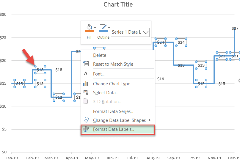
How to Create a Step Chart in Excel - Automate Excel

How to add data labels from different columns in an Excel chart? Step 5. To add data labels, right-click the set of data in the chart, then pick the Add Data Labels option in Add Data Labels from the context menu. This will bring up a new window. Step 6. This is the data label that is currently shown in the chart. Step 7. If you click any data label, then all data labels will be selected.

Enable or Disable Excel Data Labels at the click of a button - How To - PakAccountants.com

Data Labels in Excel Pivot Chart (Detailed Analysis) Next open Format Data Labels by pressing the More options in the Data Labels. Then on the side panel, click on the Value From Cells. Next, in the dialog box, Select D5:D11, and click OK. Right after clicking OK, you will notice that there are percentage signs showing on top of the columns. 4. Changing Appearance of Pivot Chart Labels

Enable or Disable Excel Data Labels at the click of a button - How To - PakAccountants.com

Add or remove data labels in a chart - support.microsoft.com Click the data series or chart. To label one data point, after clicking the series, click that data point. In the upper right corner, next to the chart, click Add Chart Element > Data Labels. To change the location, click the arrow, and choose an option. If you want to show your data label inside a text bubble shape, click Data Callout.

How to Make a Bar Chart in Excel | Smartsheet

How to Place Labels Directly Through Your Line Graph in Microsoft Excel Right-click on top of one of those circular data points. You'll see a pop-up window. Click on Add Data Labels. Your unformatted labels will appear to the right of each data point: Click just once on any of those data labels. You'll see little squares around each data point. Then, right-click on any of those data labels. You'll see a pop-up menu.

Data labels on Excel charts « projectwoman.com

How To Add Data Labels In Excel " .paymycheck Then, click the insert tab along the top ribbon and click the insert scatter (x,y) option in the charts group. Click on the arrow next to data labels to change the position of where the labels are in relation to the bar chart. To format data labels in excel, choose the set of data labels to format. Source:

30 What Is A Data Label In Excel - Labels Database 2020

How to use data labels in a chart - YouTube Excel charts have a flexible system to display values called "data labels". Data labels are a classic example a "simple" Excel feature with a huge range of o...

Change Column Colors / Show Percent Labels in Excel Column Chart

How to Use Cell Values for Excel Chart Labels - How-To Geek Select the chart, choose the "Chart Elements" option, click the "Data Labels" arrow, and then "More Options." Uncheck the "Value" box and check the "Value From Cells" box. Select cells C2:C6 to use for the data label range and then click the "OK" button. The values from these cells are now used for the chart data labels.

How to Create a Bar Chart With Labels Above Bars in Excel

How to make a pie chart in Excel - Ablebits Nov 12, 2015 · Adding data labels to a pie chart; Showing data categories on the labels; Excel pie chart percentage and value; Adding data labels to Excel pie charts. In this pie chart example, we are going to add labels to all data points. To do this, click the Chart Elements button in the upper-right corner of your pie graph, and select the Data Labels ...

How-to Put Percentage Labels on Top of a Stacked Column Chart - Excel Dashboard Templates

Edit titles or data labels in a chart - support.microsoft.com On a chart, click one time or two times on the data label that you want to link to a corresponding worksheet cell. The first click selects the data labels for the whole data series, and the second click selects the individual data label. Right-click the data label, and then click Format Data Label or Format Data Labels.

Share :