41 excel pivot table conditional formatting row labels
Excel Pivot Table Macro Paste Format Values Follow these steps to copy a pivot table's values and formatting: Select the original pivot table, and copy it. Click the cell where you want to paste the copy. On the Excel Ribbon's Home tab, click the Dialog Launcher button in the Clipboard group . In the Clipboard, click on the pivot table copy, in the list of copied items.. sfmagazine.com › post-entry › april-2017-excelEXCEL: SETTING PIVOT TABLE DEFAULTS - Strategic Finance Apr 01, 2017 · Open the workbook that contains the pivot table. Select one cell in the pivot table. Go to File, Options, Advanced, Data, and click the button for Edit Default Layout. Use the Layout Import feature by entering a single cell from the pivot table in Layout Import and clicking the Import button. All of the settings from the pivot table will become ...
How to Apply Conditional Formatting to Pivot Tables - Excel … 13/12/2018 · Bottom Line: Learn how to apply conditional formatting to pivot tables so that the formats are dynamically reapplied as the pivot table is changed, filtered, or updated. Skill Level: Intermediate Download the Excel File. Here's the file that I use in the video. You can use it to practice adding, deleting, and changing conditional formatting on a variety of pivot table …
Excel pivot table conditional formatting row labels
trumpexcel.com › group-numbers-in-pivot-tableHow to Group Numbers in Pivot Table in Excel You May Also Like the Following Pivot Table Tutorials: How to Group Dates in Pivot Table in Excel. How to Create a Pivot Table in Excel. Preparing Source Data For Pivot Table. How to Refresh Pivot Table in Excel. Using Slicers in Excel Pivot Table – A Beginner’s Guide. How to Apply Conditional Formatting in a Pivot Table in Excel. The Pivot table tools ribbon in Excel These two tabs allow you to perform pivot table customization. This is the Pivot table ribbon in Excel. Create pivot table fields , charts and sets. Here is an important thing to wonder for the pivot table ribbon in excel is as soon as you switch the selected cell to non pivot table cell. The pivot table ribbon disappears. So it means Excel ... How to Delete a PivotTable in Microsoft Excel Like this, it's also quick and easy to remove blank rows and columns in Excel. RELATED: How to Quickly and Easily Delete Blank Rows and Columns in Excel. Remove a PivotTable Using a Ribbon Option. Another way to clear a PivotTable in your spreadsheet is to use an option in Excel's ribbon. To use this method, first, click any cell in your ...
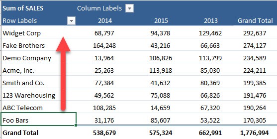
Excel pivot table conditional formatting row labels. How To Compare Multiple Lists of Names with a Pivot Table - Excel Campus 08/07/2014 · Column E of the Pivot Table contains the Grand Total (sum of columns B:D). People that volunteered all three years will have a “3” in column E. We should sort the pivot table so all the people with a “3” in column E appear at the top of the list. This will make it … › documents › excelHow to remove bold font of pivot table in Excel? - ExtendOffice The normal Bold feature can’t help us to un-bold the row labels in pivot table, but we can apply the powerful function – Conditional Formatting to solve this problem. Please do as follows: 1. Select the bold font row you want to un-bold in the pivot table, or you can press Ctrl key to select multiple bold font rows as your need. See screenshot: Merge two relational data sets - Get Digital Help 4. Set up Pivot Table. The image above shows a Pivot Table to the left and the corresponding task pane to the right. The task pane contains a list of fields based on headers in your Excel Table, you can drag these fields to different areas below which are: Report Filter; Column Labels (horizontally) Row Labels (vertically) Values r - Nested Row Labels to Column - Stack Overflow Nested Row Labels to Column. I have a CSV that appears to be the output of an Excel Pivot Table with names nested as row labels for repeating groups. I would like to clean the data so that the row labels are repeated in a separate column, ideally using dplyr. dd <- data.frame (variables = c ("Abington", "Number of Sales","YTD Number of Sales ...
Excel Pivot Table Formatting (The Ultimate Guide) - ExcelDemy First, select the entire Pivot table and click on the right button of your mouse to press the Format Cells option. In the protection option of the Format Cells box. Uncheck the Locked option and press OK. Then on the Review Tab on top click on the Protect Sheet option Put a tick mark on the Select unlocked cells and set a password. linkedin-skill-assessments-quizzes/microsoft-excel-quiz.md at ... - GitHub In the cells group on the Home tab, click Format > Format Cells. Then click the Alignment tab and select Right Indent. Click the Decrease Decimal button once. Q13. Which formula is NOT equivalent to all of the others? =A3+A4+A5+A6 =SUM (A3:A6) =SUM (A3,A6) =SUM (A3,A4,A5,A6) Q14. EXCEL: SETTING PIVOT TABLE DEFAULTS - Strategic Finance 01/04/2017 · The second way to set the defaults is useful if you have a pivot table that’s already in the correct format. You can base the defaults on that pivot table. Open the workbook that contains the pivot table. Select one cell in the pivot table. Go to File, Options, Advanced, Data, and click the button for Edit Default Layout. 101 Advanced Pivot Table Tips And Tricks You Need To Know 25/04/2022 · Without a table your range reference will look something like above. In this example, if we were to add data past Row 51 or Column I our pivot table would not include it in the results. To create and name your table. Select your data. Go to the Insert tab and press the Table button in the Tables section, or use the keyboard shortcut Ctrl + T.
How to Format Excel Pivot Table - Contextures Excel Tips Follow these steps to copy a pivot table's values and formatting: Select the original pivot table, and copy it. Click the cell where you want to paste the copy. On the Excel Ribbon's Home tab, click the Dialog Launcher button in the Clipboard group . In the Clipboard, click on the pivot table copy, in the list of copied items.. find and highlight a list of values in excel find and highlight a list of values in excel. what does the pregnant emoji mean on tiktok; what languages does alvaro soler speak; why did maude keep her neck covered How to Group Numbers in Pivot Table in Excel You May Also Like the Following Pivot Table Tutorials: How to Group Dates in Pivot Table in Excel. How to Create a Pivot Table in Excel. Preparing Source Data For Pivot Table. How to Refresh Pivot Table in Excel. Using Slicers in Excel Pivot Table – A Beginner’s Guide. How to Apply Conditional Formatting in a Pivot Table in Excel. Excel Pivot Tables - by contextures.com You can use conditional formatting in an Excel pivot table, to highlight specific data, such as months with high sales numbers. This example uses conditional formatting to highlight the pivot table values that are connected to weekend dates. Continue reading March 9, 2022 Formatting Leave a comment
Sorting a Pivot Table | MyExcelOnline
How to add conditional formatting to Excel PivotTable in 3 easy steps This approach will be flexible for variable rows and columns. 1. Select any calculated cell in PivotTable. 2. Go to the Conditional Formatting tool in the Excel Home tab and choose one of the options. 3. Look at the right side of the previously selected PivotTable cell. You will see a little icon. Choose how to apply conditional formatting.

26 MS Excel ideas | excel, excel shortcuts, pivot table
EOF
Rename Pivot Table | Decorations I Can Make
How to Show Text in Pivot Table Values Area - Contextures Excel … 27/01/2022 · There are special settings to use when you apply conditional formatting in a pivot table. To change the region numbers to text, follow these steps to manually add conditional formatting: Select all the Value cells in the pivot table (B5:F8). NOTE: B5 is the active cell, and you can see its address in the NameBox

How to achieve RFM analysis model with EXCEL - Programmer Sought
› excel-pivot-tables › the-pivotThe Pivot table tools ribbon in Excel These two tabs allow you to perform pivot table customization. This is the Pivot table ribbon in Excel. Create pivot table fields , charts and sets. Here is an important thing to wonder for the pivot table ribbon in excel is as soon as you switch the selected cell to non pivot table cell. The pivot table ribbon disappears.

How To Find And Remove Duplicates In A Pivot Table - MS Excel | Excel In Excel
Advanced Microsoft Excel 2016 | Community Care Alliance Develop essential skills in Microsoft Excel 2016 to better consolidate, analyze, and report on data. This course provides expert instruction and hands-on exercises that will help you easily master analysis tools, PivotTables, conditional formatting, and other advanced features. 6 Weeks Access / 24 Course Hrs.

33 Pivot Table Blank Row Label - Labels Database 2020
How to Calculate Percentage in a Pivot Table - Excel Exercise Adding percentage to a pivot table it's very easy. Drag and drop the same field 2 times Click on the arrow (on the left of the field) Select the option Value Field Settings In the dialog box, select the tab Show Values As Then, in the dropdown list, you select % of Grand Total AND THAT'S ALL ! Percentage parent

How to Create a MS Excel 2010 Pivot Table – An Introduction | Technical Communication Center ...
How to Highlight Active Row in Excel (3 Methods) - ExcelDemy At this step, Right click on the sheet name ( CF & VBA) where you want to highlight the active row. It will open the VBA window. In this VBA window, you will see the Code window of that sheet. Type the following code in the Code window, Private Sub Worksheet_SelectionChange(ByVal Target As Range) With ThisWorkbook.Names("HighlightActiveRow ...

How to Apply Data Bars in Pivot Table - MS Excel | Excel In Excel
101 Excel Pivot Tables Examples | MyExcelOnline 31/07/2020 · Pivot Tables in Excel are one of the most powerful features within Microsoft Excel. An Excel Pivot Table allows you to analyze more than 1 million rows of data with just a few mouse clicks, show the results in an easy to read table, “pivot”/change the report layout with the ease of dragging fields around, highlight key information to management and include Charts & …
Post a Comment for "41 excel pivot table conditional formatting row labels"