41 excel chart with labels from data
How to Add Data Labels in Excel - Excelchat | Excelchat After inserting a chart in Excel 2010 and earlier versions we need to do the followings to add data labels to the chart; Click inside the chart area to display the Chart Tools. Figure 2. Chart Tools. Click on Layout tab of the Chart Tools. In Labels group, click on Data Labels and select the position to add labels to the chart. Change the format of data labels in a chart To get there, after adding your data labels, select the data label to format, and then click Chart Elements > Data Labels > More Options. To go to the appropriate area, click one of the four icons ( Fill & Line, Effects, Size & Properties ( Layout & Properties in Outlook or Word), or Label Options) shown here.
Custom Chart Data Labels In Excel With Formulas Follow the steps below to create the custom data labels. Select the chart label you want to change. In the formula-bar hit = (equals), select the cell reference containing your chart label's data. In this case, the first label is in cell E2. Finally, repeat for all your chart laebls.

Excel chart with labels from data
How To Add Data Labels In Excel : deiseanimalsanctuary First add data labels to the chart (layout ribbon > data labels) define the new data label values in a bunch of cells, like this: Select the chart label you want to change. Source: superuser.com. Data labels make an excel chart easier to understand because they show details about a data series or its individual data points. Click the chart to ... Excel charts: add title, customize chart axis, legend and data labels ... Click the Chart Elements button, and select the Data Labels option. For example, this is how we can add labels to one of the data series in our Excel chart: For specific chart types, such as pie chart, you can also choose the labels location. For this, click the arrow next to Data Labels, and choose the option you want. Excel: How to Create a Bubble Chart with Labels - Statology Step 3: Add Labels. To add labels to the bubble chart, click anywhere on the chart and then click the green plus "+" sign in the top right corner. Then click the arrow next to Data Labels and then click More Options in the dropdown menu: In the panel that appears on the right side of the screen, check the box next to Value From Cells within ...
Excel chart with labels from data. How to use cell values for excel chart labels - How to This method will guide you to manually add a data label from a cell of different column at a time in an Excel chart. 1 . Right click the data series in the chart, and select Add Data Labels > Add Data Labels How to add data labels from different column in an Excel chart? Right click the data series in the chart, and select Add Data Labels > Add Data Labels from the context menu to add data labels. 2. Click any data label to select all data labels, and then click the specified data label to select it only in the chart. 3. Creating a chart with dynamic labels - Microsoft Excel 2016 1. Right-click on the chart and in the popup menu, select Add Data Labels and again Add Data Labels : 2. Do one of the following: For all labels: on the Format Data Labels pane, in the Label Options, in the Label Contains group, check Value From Cells and then choose cells: For the specific label: double-click on the label value, in the popup ... Add a DATA LABEL to ONE POINT on a chart in Excel Method — add one data label to a chart line Steps shown in the video above: Click on the chart line to add the data point to. All the data points will be highlighted. Click again on the single point that you want to add a data label to. Right-click and select ' Add data label ' This is the key step!
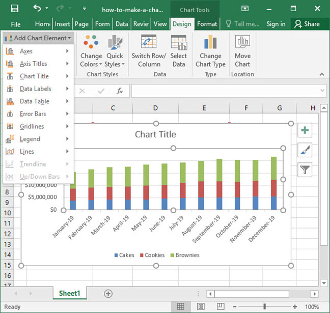
How to Place Labels Directly Through Your Line Graph in Microsoft Excel Right-click on top of one of those circular data points. You'll see a pop-up window. Click on Add Data Labels. Your unformatted labels will appear to the right of each data point: Click just once on any of those data labels. You'll see little squares around each data point. Then, right-click on any of those data labels. You'll see a pop-up menu. Add / Move Data Labels in Charts - Excel & Google Sheets We'll start with the same dataset that we went over in Excel to review how to add and move data labels to charts. Add and Move Data Labels in Google Sheets Double Click Chart Select Customize under Chart Editor Select Series 4. Check Data Labels 5. Select which Position to move the data labels in comparison to the bars. Add or remove data labels in a chart - support.microsoft.com Click the data series or chart. To label one data point, after clicking the series, click that data point. In the upper right corner, next to the chart, click Add Chart Element > Data Labels. To change the location, click the arrow, and choose an option. If you want to show your data label inside a text bubble shape, click Data Callout. The Tested and Proven Chart Add-in for Excel Open the worksheet and click the Insert menu button. From Insert menu click the My Apps button to access the ChartExpo add-in. Select ChartExpo and click the Insert button to get started with ChartExpo. Click the Search Box and type your preferred chart.
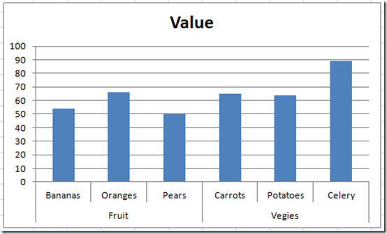
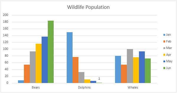
How to Create a Bar Chart With Labels Above Bars in Excel In the Format Data Labels pane, under Label Options selected, set the Label Position to Inside End. 16. Next, while the labels are still selected, click on Text Options, and then click on the Textbox icon. 17. Uncheck the Wrap text in shape option and set all the Margins to zero. The chart should look like this: 18. Example: Charts with Data Labels - XlsxWriter Documentation A demo of some of the Excel chart data labels options that are available via an XlsxWriter chart. These include custom labels with user text or text taken from cells in the worksheet. See also Chart series option: Data Labels and Chart series option: Custom Data Labels. Chart 1 in the following example is a chart with standard data labels: How to Create Charts in Excel (In Easy Steps) 1. Select the chart. 2. On the Design tab, in the Type group, click Change Chart Type. 3. On the left side, click Column. 4. Click OK. Result: Switch Row/Column If you want to display the animals (instead of the months) on the horizontal axis, execute the following steps. 1. Select the chart. 2. How to Create a Bar Chart With Labels Inside Bars in Excel In the chart, right-click the Series "# Footballers" Data Labels and then, on the short-cut menu, click Format Data Labels. 8. In the Format Data Labels pane, under Label Options selected, set the Label Position to Inside End. 9. Next, in the chart, select the Series 2 Data Labels and then set the Label Position to Inside Base. 10.
Excel Dashboard Templates Fixing Your Excel Chart When the Multi-Level Category Label Option is ...
How To Use Dynamic Data Labels To Create Interactive Excel Charts Insert An Interactive Line Chart With Dynamic Data Labels Select the data and insert a combo chart. For combo, chart go to the Insert → Charts → Combo Charts Now make a selection for the Line Chart for revenue data and a Line Chart With Markers For Data Labels. Now select the Data Label Line and remove fill color from it.

Excel Course: Inserting Graphs
Excel Charts - Aesthetic Data Labels - Tutorials Point Data labels stay in place, even when you switch to a different type of chart. You can also connect the data labels to their data points with leader lines on all charts. Here, we will use a Bubble chart to see the formatting of data labels. Data Label Positions. To place the data labels in the chart, follow the steps given below.
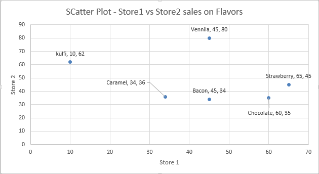
Add Custom Labels to x-y Scatter plot in Excel - DataScience Made Simple
Add data labels and callouts to charts in Excel 365 | EasyTweaks.com Step #1: After generating the chart in Excel, right-click anywhere within the chart and select Add labels . Note that you can also select the very handy option of Adding data Callouts. Step #2: When you select the "Add Labels" option, all the different portions of the chart will automatically take on the corresponding values in the table ...
How To Make a Chart In Excel | Deskbright
How to create a chart with both percentage and value in Excel? In the Format Data Labels pane, please check Category Name option, and uncheck Value option from the Label Options, and then, you will get all percentages and values are displayed in the chart, see screenshot: 15.
Charts in Excel - Easy Excel Tutorial
How to Use Cell Values for Excel Chart Labels Select the chart, choose the "Chart Elements" option, click the "Data Labels" arrow, and then "More Options." Uncheck the "Value" box and check the "Value From Cells" box. Select cells C2:C6 to use for the data label range and then click the "OK" button. The values from these cells are now used for the chart data labels.

Show Trend Arrows in Excel Chart Data Labels
Create Dynamic Chart Data Labels with Slicers - Excel Campus You basically need to select a label series, then press the Value from Cells button in the Format Data Labels menu. Then select the range that contains the metrics for that series. Click to Enlarge Repeat this step for each series in the chart. If you are using Excel 2010 or earlier the chart will look like the following when you open the file.

E-xcel Tuts: Add Data Labels to Excel Charts
How do you label data points in Excel? - profitclaims.com 1. Right click the data series in the chart, and select Add Data Labels > Add Data Labels from the context menu to add data labels. 2. Click any data label to select all data labels, and then click the specified data label to select it only in the chart. 3.

How to Make Charts and Graphs in Excel | Smartsheet
How to create Custom Data Labels in Excel Charts Right click on any data label and choose the callout shape from Change Data Label Shapes option. Now adjust each data label as required to avoid overlap. Put solid fill color in the labels Finally, click on the chart (to deselect the currently selected label) and then click on a data label again (to select all data labels).

Creating Pie Chart and Adding/Formatting Data Labels (Excel) - YouTube
How to Add Labels to Scatterplot Points in Excel - Statology Step 3: Add Labels to Points. Next, click anywhere on the chart until a green plus (+) sign appears in the top right corner. Then click Data Labels, then click More Options…. In the Format Data Labels window that appears on the right of the screen, uncheck the box next to Y Value and check the box next to Value From Cells.

Improve your X Y Scatter Chart with custom data labels
Excel: How to Create a Bubble Chart with Labels - Statology Step 3: Add Labels. To add labels to the bubble chart, click anywhere on the chart and then click the green plus "+" sign in the top right corner. Then click the arrow next to Data Labels and then click More Options in the dropdown menu: In the panel that appears on the right side of the screen, check the box next to Value From Cells within ...

How to Change Data Label in Chart / Graph in MS Excel 2013 - YouTube
Excel charts: add title, customize chart axis, legend and data labels ... Click the Chart Elements button, and select the Data Labels option. For example, this is how we can add labels to one of the data series in our Excel chart: For specific chart types, such as pie chart, you can also choose the labels location. For this, click the arrow next to Data Labels, and choose the option you want.

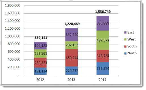
Excel-User.com: Excel Charts - Add totals labels to Stacked Column chart
How To Add Data Labels In Excel : deiseanimalsanctuary First add data labels to the chart (layout ribbon > data labels) define the new data label values in a bunch of cells, like this: Select the chart label you want to change. Source: superuser.com. Data labels make an excel chart easier to understand because they show details about a data series or its individual data points. Click the chart to ...
How to Show Percentages in Stacked Bar and Column Charts in Excel
How-to Add Custom Labels that Dynamically Change in Excel Charts - Excel Dashboard Templates
Bar Chart in Excel - Easy Excel Tutorial
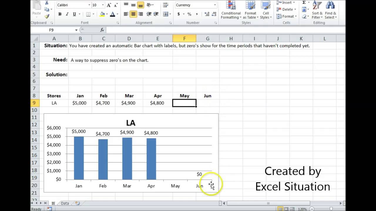
Excel Bar Chart Suppress Zeros - YouTube
Format Number Options for Chart Data Labels in Excel 2011 for Mac

Excel 2010 pie chart data labels in case of "Best Fit"
Post a Comment for "41 excel chart with labels from data"