38 use the format data labels task pane to display category name and percentage data labels

Change the format of data labels in a chart To get there, after adding your data labels, select the data label to format, and then click Chart Elements > Data Labels > More Options. To go to the appropriate area, click one of the four icons ( Fill & Line, Effects, Size & Properties ( Layout & Properties in Outlook or Word), or Label Options) shown here. A data label is descriptive text that shows that exact value or name of ... To format the data labels - Double click a data label to open the Format Data Labels task pane. Click the Label Options Icon. Click Label Options to customize the labels, and complete any of the following steps: Select the Label Contains options. The default is Value, but you might want to display additional label contents, such as Category Name.

Airline Arrivals Analysis | Sample Assignment Right-click one of the data labels and select Format Data Labelsto open the Format Data Label task pane. Click Label Options, click the Percentage check boxto select it, and then click the Value check box to deselect it. Close the Format Data Labels task pane. Typically, pie chart data labels show percentages instead of values.

Use the format data labels task pane to display category name and percentage data labels

UsetheFormatDataLabelstaskpanetodisplay - Course Hero Apply 18 point size to the data labels. a. Click green plus data labels center click green plus double click in chart label contains click percentage click values check box click close click home font 18 9. Open the Format Chart Area task pane. Apply the Blue tissue paper texture fill to the chart area of the pie chart. Keep the task pane open. Excel charts: add title, customize chart axis, legend and data labels ... Click anywhere within your Excel chart, then click the Chart Elements button and check the Axis Titles box. If you want to display the title only for one axis, either horizontal or vertical, click the arrow next to Axis Titles and clear one of the boxes: Click the axis title box on the chart, and type the text. Formatting Data Labels - BusinessView Migration Select from this drop-down menu of preset formats that can be applied to labels. Custom Format. Select this option to use a custom format. See the following table. Style Labels. Click this button to open the Style dialog box, where you can style text. The Format Labels drop-down menu provides a list of preset formats that you can apply to labels.

Use the format data labels task pane to display category name and percentage data labels. Format Data Labels in Excel- Instructions - TeachUcomp, Inc. Nov 14, 2019 · To format data labels in Excel, choose the set of data labels to format. To do this, click the “Format” tab within the “Chart Tools” contextual tab in the Ribbon. Then select the data labels to format from the “Chart Elements” drop-down in the “Current Selection” button group. Display the percentage data labels on the active chart. - YouTube Display the percentage data labels on the active chart.Want more? Then download our TEST4U demo from TEST4U provides an innovat... Solved 7 Add data labels for the % of Month line. Position - Chegg Apply 11 pt font size to the category axis, value axis, and the legend for the bar chart. 14. Use the Axis Options to display the value axis in units of Thousands, set the Major Units to 500, apply the Number format with 1 decimal place for the bar chart. Use the Axis Options to format the category axis so that the category labels are in ... 4.2 Formatting Charts - Beginning Excel, First Edition On the Design tab select the Add Chart Element button, then Data Labels, then Outside End (see Figure 4.36.) Click on one of the Data Labels. Note that all of the data labels for that data series are selected. Using the Home ribbon, change the font to Arial, Bold, size 9. Click on one of the data labels for the other data series.

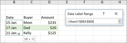
Add or remove data labels in a chart - support.microsoft.com Right-click the data series or data label to display more data for, and then click Format Data Labels. Click Label Options and under Label Contains, select the Values From Cells checkbox. When the Data Label Range dialog box appears, go back to the spreadsheet and select the range for which you want the cell values to display as data labels. Excel Module 4 Flashcards | Quizlet you want to show the percentages only, not their numerical values.in the task pane, in the label contains section, click the value check box to deselect it.excel removes the numerical values from the data labels.in the label position section, click the inside end option button to select it.excel moves the data labels to the inside end position.in … Excel 3-D Pie charts - Microsoft Excel 2016 - OfficeToolTips If you want to create a pie chart that shows your company (in this example - Company A) in the greatest positive light: Do the following: 1. Select the data range (in this example, B5:C10 ). 2. On the Insert tab, in the Charts group, choose the Pie button: Choose 3-D Pie. 3. Right-click in the chart area, then select Add Data Labels and click ... How do you format data series in Excel? - FAQ-ALL Select the decimal number cells, and then click Home > % to change the decimal numbers to percentage format . 7. Then go to the stacked column, and select the label you want to show as percentage , then type = in the formula bar and select percentage cell, and press Enter key. How to format data series independently in Excel

cs 385 exam 3 Flashcards - Quizlet data tab, subtotal, click at each change in: select area, unselect replace current subtotals, click ok Collapse the table to show the grand totals only. click 1 at top left corner Expand the table to show the grand and discipline totals. click 2 at top left corner Use the Auto Outline feature to group the columns. How to show data label in "percentage" instead of - Microsoft Community Jul 05, 2012 · Select Format Data Labels Select Number in the left column Select Percentage in the popup options In the Format code field set the number of decimal places required and click Add. (Or if the table data in in percentage format then you can select Link to source.) Click OK Regards, OssieMac Report abuse 8 people found this reply helpful · How to create a chart with both percentage and value in Excel? Then, please go on right click the bar, and select Format Data Labels option, see screenshot: 14. In the Format Data Labels pane, please check Category Name option, and uncheck Value option from the Label Options, and then, you will get all percentages and values are displayed in the chart, see screenshot: 15. Solved step by step instruction 2 A pie chart is an | Chegg.com Use the Insert tab to create a pie chart from the Question: step by step instruction 2 A pie chart is an effective way to visually illustrate the percentage of the class that earned A, B, C, D, and F grades. Use the Insert tab to create a pie chart from the This problem has been solved! See the answer step by step instruction Expert Answer

Menambahkan atau menghapus label data dalam bagan - Dukungan Office

Excel tutorial: How to use data labels When first enabled, data labels will show only values, but the Label Options area in the format task pane offers many other settings. You can set data labels to show the category name, the series name, and even values from cells. In this case for example, I can display comments from column E using the "value from cells" option.

Hướng dẫn xây dựng biểu đồ hình tròn trong Excel, nhiều kỹ thuật hay và hữu ích.

How to: Display and Format Data Labels - DevExpress In particular, set the DataLabelBase.ShowCategoryName and DataLabelBase.ShowPercent properties to true to display the category name and percentage value in a data label at the same time. To separate these items, assign a new line character to the DataLabelBase.Separator property, so the percentage value will be automatically wrapped to a new line.

Share :